Training a drive-failure model on a GPU server's CPU
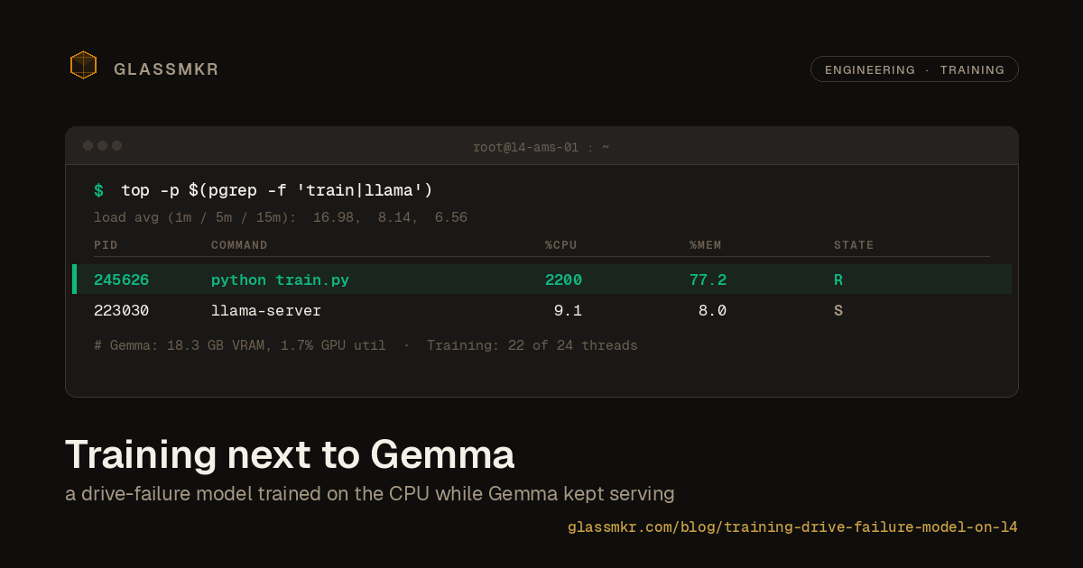
We retrained a drive-failure predictor on two years of Backblaze data without renting any extra compute. The model trained on the CPU of the same L4 GPU server that runs Furnace, our self-hosted Gemma 4 inference on an NVIDIA L4 in Amsterdam, while Gemma stayed resident in VRAM and kept answering requests. Total wall-clock: 59 minutes for 222 million drive-days of training data. Gemma's latency was 5.8% slower during training. No new cloud bill, no separate training node, no moving the model off-box.
This post walks through what that setup looked like, why it works, and what the training turned up along the way. The relevant bits are the economics (you already pay for the whole machine, so use all of it), a drive-health finding that surprised us (SMART 197 beats SMART 187), and the practical limits of the approach (don't try this on a 16 GB laptop).
Why retraining costs nothing extra
The Furnace box (L4 GPU + AMD EPYC 4464P) is 12 Zen 4 cores, 24 threads, 64 GB of RAM, sitting in Amsterdam on a private WireGuard mesh. During normal operation, the L4's 24 GB of VRAM is pinned to Gemma, and the GPU itself is only busy when an inference request comes in. The CPU sits at single-digit utilization most of the time, serving only the orchestration of llama.cpp request handling.
Which means there's an entire 24-thread workstation sitting idle on the same box where our production LLM runs. We already paid for it.
For a quarterly retraining of our drive-failure model, that idle CPU is exactly the right resource. The training isn't a continuous workload. It runs once a quarter, takes an hour, and then the hardware goes back to what it was doing. If we had to provision a separate training box for this (or rent a cloud instance), we'd be paying for compute that sits idle 24 hours a day, 89 days out of 90. Instead we use the CPU we already have.
The constraint is that the training must not disturb the inference workload. VRAM pressure is out of the question; Gemma uses 18.3 GB of the L4's 24 GB and we can't afford swap. CPU contention has to be bounded too, because even though llama.cpp does its heavy lifting on the GPU, it still needs cores for request handling, prompt processing, and the pre- and post-steps of inference.
The question this post answers is whether a real training job actually satisfies those constraints in practice, not just in theory.
The job
Backblaze publishes a quarterly drive-failure dataset: CSV files, one row per drive per day, with SMART attributes and a failure flag on the day a drive dies. We used Q1 2024 through Q4 2025, which unpacks to 82 GB across 731 CSV files covering 222,773,948 drive-days and 259,648 failure events across 374,869 unique drives. Temporal split: everything before July 2025 is training, everything after is held-out validation.
The target is a LightGBM classifier that predicts whether a drive will fail within 30 days, given SMART attributes and their recent trends. It's used in Dashboard's Stage 2.5 tier ranker, which adjusts alert severity on known-degrading drives. A model score above 0.7 tiers an alert up; below 0.1 can tier it down. Everything in between defers to the rules engine.
The pipeline has four steps:
prepare_features.py: stream the CSVs through DuckDB, sort by (serial, date), compute lagged deltas and rolling windows for SMART attributes, write a Parquet file.train.py: load Parquet, apply negative subsampling (keep all 259k positives plus a 5% uniform sample of the 222M negatives), train a LightGBM booster with early stopping.validate.py: score the full 60.8M-row held-out validation set (no subsampling here), compute AUROC, PR curve, per-vendor breakdown.export_onnx.py: convert the booster to ONNX, verify parity against the original on 1000 random rows.
All four steps ran serially on the L4 server's CPU while the L4 itself stayed pinned to Gemma.
What the GPU did for 59 minutes
Sampling GPU state every 5 seconds for the duration of the training run: VRAM held at 18.3 GB, with a total drift of 30 MiB across 711 samples. That 30 MiB isn't training. It's Gemma's KV cache growing as inference requests came in. Training allocated nothing on the GPU. Not a stray tensor, not a scratch buffer. LightGBM doesn't use CUDA.
GPU utilization averaged 1.7% during training. The peaks hit 98%, but only in the brief windows when Gemma served an inference request. The baseline state was a GPU resident with Gemma's weights, idling, waiting.
This is the point: the training job was running full-tilt on the CPU (22 of 24 threads saturated during the LightGBM boosting loop), while the GPU had no idea anything unusual was happening. The two workloads compete for different hardware. CPU cores for training, GPU SMs for inference. They don't fight.
Did Gemma slow down?
To test this empirically rather than just by argument, we triggered three Gemma inference requests from a separate SSH session during the train.py window, when all 24 CPU threads were at 100%. These are the same kind of requests Gemma serves in production: ~6500 input tokens, structured JSON output, same system prompt as the Qwen benchmark.
| Gemma run during training | Elapsed | Valid JSON | Findings |
|---|---|---|---|
| 1 | 22.41 s | yes | 4 |
| 2 | 15.98 s | yes | 4 |
| 3 | 12.91 s | yes | 3 |
| Average | 17.10 s | 3/3 | 3.67 |
Idle baseline from our Qwen vs Gemma benchmark was 16.16 s (average of 3 runs). So Gemma during training averaged 17.10 s vs 16.16 s at baseline: a 5.8% latency increase.
Caveat: three samples is a tiny comparison. The Qwen benchmark's idle runs ranged from 13.74 s to 17.66 s, so any one of our training-window runs could plausibly sit anywhere in that band. The 5.8% overhead is inside normal run-to-run variance, which is the claim worth making. What we can say with confidence is that Gemma stayed functional, all outputs were valid JSON with the expected finding counts, and nothing in the observed latencies would be visible to a Dashboard user watching a health analysis render. What we can't say is "0% overhead" or "never degrades under load." At a higher concurrent inference rate or longer sustained training windows, this might be different.
What we can also say: the training job peaked at 2200% CPU (22 threads at 100%) while llama.cpp stayed at 9% CPU. Both co-existed because they were asking for different resources.
The feature ranking surprised us
The research hypothesis going in, based on Backblaze's own blog posts and the operator folklore that grew around them, was that SMART 187 (Reported Uncorrectable Errors) would be the dominant feature. It wasn't.
| Rank | Feature | % of total gain |
|---|---|---|
| 1 | smart_197_raw | 25.3% |
| 2 | smart_5_raw | 20.1% |
| 3 | model_afr_prior | 10.8% |
| 4 | drive_age_days | 8.4% |
| 5 | smart_187_raw | 6.7% |
| 6 | smart_197_delta_30d | 6.3% |
| 7 | smart_5_delta_30d | 5.7% |
SMART 197 (Current Pending Sector Count) topped the ranking at 25.3% of total gain, followed by SMART 5 (Reallocated Sector Count) at 20.1%. SMART 187 landed fifth.
This contradicts a widely-repeated piece of operator advice, which is worth addressing carefully. The claim isn't that SMART 187 is useless. It's still a strong individual indicator, and if you only get to alert on one SMART attribute, it's defensible. The claim is that when you combine 27 features in a boosted tree, the marginal information content of SMART 197 exceeds SMART 187's. This is consistent with Botezatu et al. (2016), who found pending-sector count outperforms reported-uncorrectable on 30-day-horizon prediction tasks. Backblaze's own analysis leans on SMART 187 in part because of how their monitoring surfaces it in isolation, not because it's the most predictive attribute in a combined model.
The practical implication for a rules engine isn't "alert on 197 instead of 187." Both still matter. The implication is for tier-ranker training: when you're picking which features to engineer deltas and rolling windows for, 197 should be at the top of the list, not 187. It is for us.
The drive_age_days feature at 8.4% is worth noting too. Older drives fail more. This isn't news, but it's useful confirmation that the model is catching the AFR (Annual Failure Rate) curve correctly rather than learning shortcuts from serial-number patterns. The per-model AFR prior at 10.8% similarly confirms that drive model identity carries legitimate signal, not just leakage.
Validation
AUROC on the full held-out validation set was 0.8864. The spec aimed for 0.90, so we're just short. Context for that:
Published benchmarks like DFPoLD and RODMAN report AUROC in the 0.89 to 0.94 range on similar data. Those papers aggregate predictions to drive-week, which means a single prediction per drive per week rather than one per drive per day. Aggregation shifts the positive base rate and inflates AUROC. Our validation is at the row level (one prediction per drive-day), which is closer to how the tier ranker actually runs in production. A like-for-like row-level evaluation of DFPoLD's method would likely land closer to our 0.886 than to their 0.94.
The PR-curve operating points look bad at first glance:
| FPR | Precision | Recall | TP | FP |
|---|---|---|---|---|
| 0.1% | 9.83% | 11.4% | 6,478 | 59,425 |
| 0.5% | 6.38% | 36.4% | 20,673 | 303,190 |
| 0.8% | 4.85% | 43.5% | 24,734 | 485,648 |
| 2.0% | 2.57% | 56.3% | 31,978 | 1,212,754 |
The spec (copied from DFPoLD/RODMAN) targets precision above 75% at 0.8% FPR. We got 4.85%. That's not a model failure; it's a base-rate ceiling. At 0.094% positive rate, even a perfect classifier bounds precision at 0.8% FPR to about 10.5%. To get 75% precision at that FPR on this base rate, you would need the classifier to achieve near-perfect ranking of all 56,837 failures within the top 456,000 scored rows out of 60.8 million. No classifier on this dataset does that. The 75% number in the spec assumes drive-week aggregation, which shifts the base rate roughly 7-fold and makes those operating points reachable.
For the Stage 2.5 tier ranker, AUROC is the right quality metric because the ranker only tiers alerts up at score > 0.7 (high confidence failure) or down at score < 0.1 (high confidence healthy). It doesn't operate at arbitrary FPR points. AUROC 0.886 is a perfectly usable operating characteristic at those score thresholds, and it's what validate.py hard-fails on.
Per-vendor AUROC tells a more textured story:
| Vendor | Drive-days | Failures | AUROC |
|---|---|---|---|
| Seagate | 20.9M | 21,650 | 0.9035 |
| WDC | 14.7M | 6,817 | 0.8746 |
| Toshiba | 20.0M | 19,165 | 0.8524 |
| HGST/Hitachi | 5.0M | 9,186 | 0.8301 |
Seagate is the easiest to predict, HGST is hardest. This matches Backblaze's own observation that older Hitachi drives often fail more abruptly, with less SMART lead time, than Seagate or WDC drives of the same generation. If we end up shipping vendor-specific score thresholds in the tier ranker later, HGST is where it would matter most. For now, the combined model is usable across all vendors.
What actually ships
The training output is a 442 KB ONNX file, a 5.8 KB metadata JSON, and a 2.4 KB per-model AFR table. Dashboard production loads all three on server startup via onnxruntime-node. The parity check between LightGBM's direct predictions and the ONNX runtime showed a maximum absolute difference of 1.02 × 10⁻⁷ across 1000 random validation rows, well inside our 1e-5 tolerance.
From snapshot arriving in Dashboard to tier-ranker score computed is a single ONNX inference call against a ~27-element float vector. No Python dependency at runtime, no PyTorch, no scikit-learn, no separate training environment. Just a small model file, a TypeScript wrapper that builds the feature vector, and the ONNX runtime.
We have written separately about why we self-host the model and how we chose it, and how Qwen3.6 benchmarks against Gemma 4 for the narration workload that shares this same L4.
Where the approach would break
This worked, but with caveats worth naming.
The training pipeline peaked at 51 GB of resident memory during the LightGBM step. That's on a 64 GB box. The first version of the pipeline used pandas for feature preparation, which tried to load the full 222M-row frame at once and OOM'd immediately. DuckDB's streaming sort and window aggregation is what made the feature-prep step fit, and even it mmapped significant temporary storage. A smaller server (for example a 16 GB box) would fail on feature prep before we ever got to training. A standard GitHub Actions runner at 7 GB will not complete this pipeline.
The 5.8% Gemma latency overhead was measured on three requests. Scale and sustained load could look different. Real production inference is close to serial in our setup (one analysis every 60 seconds per server), so high concurrent inference collisions with training are rare by design. If they mattered, we could gate the training job to low-traffic windows. We didn't need to.
DuckDB's 53-minute feature-prep step was slower than our earlier ad-hoc benchmark runs of the same code. The difference was that during this run, the GPU sampler was running, llama.cpp was serving Gemma, and the three benchmark Gemma requests consumed some cores. Co-location isn't free in the feature-prep step, even if it's effectively free at the GPU level. That's a reasonable trade for us; the job still finishes in an hour and we didn't need to pay for anything extra.
Using what you own
The architectural point is the one worth leaving with. If you run self-hosted inference on GPU hardware that isn't mostly CPU-bound, the CPU on that same box is a real resource for periodic batch workloads. Quarterly model retraining, log rollups, nightly compactions, offline analytics. Anything that's CPU-heavy, short-lived, and doesn't need its own GPU. The economics of cloud GPUs make separate training instances look reasonable. The economics of bare metal GPUs make using the CPU you already rented obvious.
We're running this job on one of our L4 servers. We expect to run the quarterly retraining on the same box for the foreseeable future. There is no separate training node in our infrastructure. There probably doesn't need to be one.